Calibration and Validation

In this section, we describe the theory behind and process of calibrating and validating the model.

Model Validation

iSDG is structured to analyze medium-long term development issues at the nationwide level, and to provide practical policy insights. Specifically, the model provides policymakers and other users with an estimate of the consequences to be expected from current and alternative policy choices. Such estimates are not to be taken as exact forecasts (no model can accurately forecast long-term development trends) but as reasonable and coherent projections, based on a set of clear and well-grounded assumptions. In fact, the model’s results inherently embed a high degree of uncertainty: over the time horizon considered in the simulation, a large variety of unforeseeable changes can take place, and a large number of parameters might take on different values than those observed in the past. The validation process of iSDG is therefore centered on strengthening the underlying assumptions based on currently available data and information, with a focus on improving its ability to provide insights in the key questions being addressed [1].

Validation is embedded in the broader model implementation process, and it includes structural and behavioral validation tests [2]. Structural validation tests involve direct verification of structural assumptions and parameters. Behavioral validation tests involve the assessment of the model’s ability to replicate the historical behavior of the main indicators for the period 2000-2020 (or latest available).

Structural validation

Testing the structural robustness of the model can be seen as consisting of five major parts [3]:

1. Qualitative structure verification: Is the model structure consistent with relevant descriptive knowledge of the system? – To answer this question, we refer you to the model documentation, which presents the descriptive knowledge of the sectors that we work with, i.e. the main assumptions about the sectors and the relevant literature justifying those assumptions. The model itself (structure and equations) can be inspected to assess the degree to which the structure is consistent with the aforementioned assumptions. The structures in the model were originally developed in line with models accepted widely in academic research and by field experts, and revisions of structures are completed in consultation with experts in those areas.

2. Extreme Conditions: Does each equation make sense even when its inputs take on extreme values? – The model is continuously subjected to such extreme condition testing, evidenced also by its application to a wide variety of economies, societies and environmental settings.

3. Boundary Adequacy (Structure): Are the important concepts for addressing the problem endogenous to the model? – For this we look at the number of SDG indicators that are reproduced endogenously in the model, and whether we can tie the performance of those indicators to policies that translate to expenditures – the analysis of which yields the cost of achieving the SDGs. Furthermore, the model should be able to link the indicators to the cost of achieving them. The iSDG achieves this through linking the policies to costed interventions which are parameterized through calibration with historical data and assumptions reviewed with relevant authorities (e.g. required per capita expenditure in health, transportation infrastructure cost per km, etc.)

4. Dimensional consistency: Is each equation dimensionally consistent? – The units used for each variable can be verified in the model. A consistency check is automatically carried out by the Stella Architect software.

5. Parameter verification: Are parameters in the model consistent with relevant descriptive (and numerical, when available) knowledge of the system? – From a pragmatic standpoint, we can verify the following categories of parameters: a. Baseline levels of indicators – to be established jointly with local experts. b. Parameters describing physical structures, such as nutrient soil dynamics or water dynamics: Based on relevant literature, each one can be seen in the model and is open to scrutiny and adjustment, as needed. c. Parameters relevant to costing, such as unit costs of infrastructure construction, and construction time – to be established jointly with local experts. d. Parameters that are established based on the calibration process. After verifying the use of the parameters, i.e. the qualitative structure verification (e.g. is there a relationship between access to roads and enrollment to schools, which in our case is expressed through an elasticity parameter?), verifying the values of the parameters is an iterative process, which is a part of the Business As Usual reporting process. In that report, the parameter combinations and the extent to which they reproduce the historical data will be detailed. The parameters can then be verified based on the summary statistics (quantitative assessment), as well as their relative sizes (qualitative assessment, e.g. verifying the relative impact of infrastructure density, governance or female participation on the total factor productivity of agriculture).

Behavioral validation

With respect to the behavioral robustness of the model, the most relevant tests for our purposes in this project are the statistical summaries provided for the indicators from all model sectors [4], which provide figures for the quantitative assessment of the degree to which the model reproduces the historical data.

The following summary statistics will be provided:

1. Population (# of historical data points)

2. Data Coverage (% of simulation points with corresponding historical data points)

3. R Squared

4. Mean Absolute Percent Error

5. Root Mean Square Error

6. Thiel Bias

7. Thiel Variation

8. Thiel Covariation

Because of the purpose of the model, the goal of calibration is that of replicating medium to long-term trends in data; while less emphasis is given to shorter term dynamics. The residual error from the calibration process is analyzed and broken down by component using Theil’s statistics [5] into bias, unequal variation, and unequal covariation. That analysis guides further calibration towards the reduction of error of the first two types in order to properly capture medium and longer-term trend in data, with less weight on error of non-systematic nature, that is due to the inability of the model to capture short-term fluctuations.

For the adequacy of these summary statistics in assessing the behavior robustness of system dynamics models see Sterman (1984) and Oliva (2003) [6].

Model Calibration

The calibration of the model takes place after the completion of the data collection process. Once the required historical time series are in place, along with any assumptions that serve to fill the remaining gaps in data, the model parameters are calibrated to the specific country context. The parameterization of any iSDG model is specific to the context and varies due to differing culture, institutions, history, demographics, economics, environment, etc. The calibration process of the model considers these differences by analyzing the historical time series (period 2000-present or latest available) and adjusting the model parameters towards those.

During the calibration process, the parameters (marked with grey in iSDG) are incrementally adjusted so that the variables down-stream in the causal chain are reproduced as closely as possible to the corresponding historical data (marked with yellow in iSDG), with a focus on medium and long-term trends. As the model consists of a large number of feedback loops (circular dynamics), the process of calibration is iterative.

The calibration takes place sector-by-sector, in the following fashion:

1. Substitute input from other sectors with historical data, thus cutting feedback loops from the sector. For example, if we are calibrating the Agriculture sector, we introduce historical data for the Land and Employment sectors.

2. Determine the available historical time-series for all of the indicators within the sector. For example, if we are calibrating the Agriculture sector, this would include crop yield, livestock production, etc.

3. Run a Powell Optimization algorithm to search for the parameter combinations that bring the model behavior closest to reproducing all of the historical indicators within the specific sector. The Powell Optimization algorithm is an efficient conjugate gradient search [7].

4. Adjust the parameters to better capture medium and longer-term trends (see summary statistics described before in the Behavioral validation section).

5. Apply the process in an iterated manner across all of the sectors. The result of the calibration process is further reviewed by local experts, and parameter values are checked against evidence from local studies. Out-of-range parameters and model behavior not in line with consensus is verified with relevant experts, as part of the BAU reporting process. Often, the initial core structure of the model, common to most applications, cannot replicate historical data sufficiently well for some indicators, indicating the need for a revision of the model’s structure and assumptions, until the proposed theory of change can explain past developments sufficiently well. This revision occurs within a participatory process with local experts.

The calibration process is based on well-established practices in System Dynamics (e.g. Homer 2012; Oliva 2003 [8]), with the following heuristics in mind:

1. Include in the calibration problem all knowledge available about the system parameters. That is, parameters which can be estimated from source material or are observable should not be optimized. As can be seen in the model, the optimized parameters are linked to social and economic functions, which are not empirically observable, and the values of which depend on the model design.

2. Apply the process to the smallest possible calibration problems. We achieve this through the sector-by-sector design of the calibration process, specifically through step 1 described above. By calibrating smaller pieces of the model, we concentrate the differences between observed and simulated behavior to those pieces of structure responsible for that behavior, thus minimizing error and maximizing structure validity.

3. Use the calibration to test the hypothesis “The estimated parameter matches the observable structure of the system”. In other words, it is not only important to reproduce the historical data, but it is also important to reproduce the historical data for the right reasons. That is, the estimated parameters must be consistent with what we know about the system. Here the participatory aspect of the calibration process comes into play, where the parameters are vetted by the relevant experts who have in-depth knowledge of and experience with the system.

Manual calibration process overview

For the focal indicator, identify the key parameters that can affect it. Adjust these parameters up or down to test the effect on the focal indicator. Adjust until a good fit is achieved with reasonable values. If values are not reasonable, further investigation is necessary, typically into the quality of the data or whether some special events have occurred that may need some special attention.

Automated calibration process overview

Stella provides optimization functions that are extensively used for calibration of iSDG. The core set of optimization files available with the model should be used throughout the calibration process (available in the core model), but can be adjusted to factor in country-specific circumstances. If the optimization file is changed, keep record of it by saving the model with a different name. When using optimization for initial rough calibration, in order to save time, typically the process can be stopped after about 100 simulations (more if using a large number of parameters). When using it for fine tuning, it is important to perform a larger number of simulations and run the process until the end. Often, manual adjustment can be used in conjunction with the automated calibration process. Additionally, ensure that there’s no strong bias towards specific parameters and that ranges and end results are within reason. If not sure of appropriate ranges, do not stray too far from the base value.

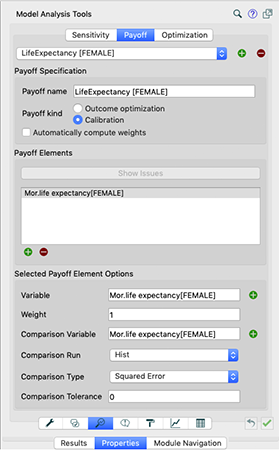
The following example explains how to use optimization and modify optimization files. Let’s say we want to optimize Average Life Expectancy. On the main model settings screen, click the lens button on the bottom. Input the settings in the Payoff tab as in the image below.

With that done, go to then to the Optimization tab and input the settings as in the image below.

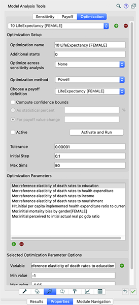
Note that the maximum simulations we’re setting to lower to start with, so that in case we have any major errors, we’re not waiting too long. These can be set higher later on for fine-tuning calibration. When finished, click OK to confirm. Then add the desired parameter ranges. In case of elasticity of mortality illustrated here, the appropriate range would be [-0.5,-0.05], different parameters would however require different ranges, and others may differ as specified below. Adjustments far out of range should be verified and noted. For example adjustment of time parameters would typically require larger positive values (for example 1,2…20 years). When satisfied with the settings, check the years of simulation and ensure they are within the range of the historical data you’re trying to match to. Then hit Run.

NB: If there are gaps in between and Stella is reading your blanks as zeros, you will need to interpolate manually in Excel.

If there’s a poor fit, there could be a problem with the input also. Caution about extremities, these may not be the ideal value, and it may be better to leave a more reasonable value than to have the perfect calibration. Additionally, with the rest of the calibration in the sector and in the model, the values would need to be adjusted later anyway.

For added insight, you may also analyze confidence bounds: a useful tool to understand how solid are calibration results.

Footnotes

[1] Forrester, J W. 1961. Industrial Dynamics. Cambridge MA: Productivity Press.

[2] Barlas, Y. 1996. “Formal Aspects of Model Validity and Validation in System Dynamics.” System Dynamics Review 12, (3): 183–210.

[3] Forrester, J W, and P M Senge. 1980. “Tests for building confidence in System Dynamics models.” TIMS Studies in the Management Sciences 14: 201–28.

Richardson, G P, and III Alexander L Pugh. 1981. Introduction to System Dynamics Modeling with Dynamo. Waltham: Pegasus Communications.

Sterman, J 2000. Business Dynamics. Irwin/McGraw-Hill.

[4] The summary statistics can be reported for any series for which we have data.

[5] Sterman, J. 1984. “Appropriate summary statistics for evaluating the historical fit of System Dynamics Models.” Dynamica 10 (2): 51–66.

[6] Sterman, J. 1984. “Appropriate summary statistics for evaluating the historical fit of System Dynamics Models.” Dynamica 10 (2): 51–66.

Oliva, R. 2003. “Model calibration as a testing strategy for System Dynamics Models.” European Journal of Operational Research 151: 553–68.

[7] Powell, M J D. 2009. The BOBYQA Algorithm for Bound Constrained Optimization Without Derivatives. Department of Applied Mathematics; Theoretical Physics, Cambridge University.

[8] Homer, J B. 2012. “Partial-model testing as a validation tool for System Dynamics (1983).” System Dynamics Review 28 (3): 281–94.

Oliva, R. 2003. “Model calibration as a testing strategy for System Dynamics Models.” European Journal of Operational Research 151: 553–68.