Calibration and Validation

In this section, we describe the theory behind and process of calibrating and validating the model.

Model Validation

iSDG is structured to analyze medium-long term development issues at the nationwide level, and to provide practical policy insights. Specifically, the model provides policymakers and other users with an estimate of the consequences to be expected from current and alternative policy choices. Such estimates are not to be taken as exact forecasts (no model can accurately forecast long-term development trends) but as reasonable and coherent projections, based on a set of clear and well-grounded assumptions. In fact, the model’s results inherently embed a high degree of uncertainty: over the time horizon considered in the simulation, a large variety of unforeseeable changes can take place, and a large number of parameters might take on different values than those observed in the past. The validation process of iSDG is therefore centered on strengthening the underlying assumptions based on currently available data and information, with a focus on improving its ability to provide insights in the key questions being addressed [1].

Validation is embedded in the broader model implementation process, and it includes structural and behavioral validation tests [2]. Structural validation tests involve direct verification of structural assumptions and parameters. Behavioral validation tests involve the assessment of the model’s ability to replicate the historical behavior of the main indicators for the period 2000-2020 (or latest available).

Structural validation

Testing the structural robustness of the model can be seen as consisting of five major parts [3]:

1. Qualitative structure verification: Is the model structure consistent with relevant descriptive knowledge of the system? – To answer this question, we refer you to the model documentation, which presents the descriptive knowledge of the sectors that we work with, i.e. the main assumptions about the sectors and the relevant literature justifying those assumptions. The model itself (structure and equations) can be inspected to assess the degree to which the structure is consistent with the aforementioned assumptions. The structures in the model were originally developed in line with models accepted widely in academic research and by field experts, and revisions of structures are completed in consultation with experts in those areas.

2. Extreme Conditions: Does each equation make sense even when its inputs take on extreme values? – The model is continuously subjected to such extreme condition testing, evidenced also by its application to a wide variety of economies, societies and environmental settings.

3. Boundary Adequacy (Structure): Are the important concepts for addressing the problem endogenous to the model? – For this we look at the number of SDG indicators that are reproduced endogenously in the model, and whether we can tie the performance of those indicators to policies that translate to expenditures – the analysis of which yields the cost of achieving the SDGs. Furthermore, the model should be able to link the indicators to the cost of achieving them. The iSDG achieves this through linking the policies to costed interventions which are parameterized through calibration with historical data and assumptions reviewed with relevant authorities (e.g. required per capita expenditure in health, transportation infrastructure cost per km, etc.)

4. Dimensional consistency: Is each equation dimensionally consistent? – The units used for each variable can be verified in the model. A consistency check is automatically carried out by the Stella Architect software.

5. Parameter verification: Are parameters in the model consistent with relevant descriptive (and numerical, when available) knowledge of the system? – From a pragmatic standpoint, we can verify the following categories of parameters: a. Baseline levels of indicators – to be established jointly with local experts. b. Parameters describing physical structures, such as nutrient soil dynamics or water dynamics: Based on relevant literature, each one can be seen in the model and is open to scrutiny and adjustment, as needed. c. Parameters relevant to costing, such as unit costs of infrastructure construction, and construction time – to be established jointly with local experts. d. Parameters that are established based on the calibration process. After verifying the use of the parameters, i.e. the qualitative structure verification (e.g. is there a relationship between access to roads and enrollment to schools, which in our case is expressed through an elasticity parameter?), verifying the values of the parameters is an iterative process, which is a part of the Business As Usual reporting process. In that report, the parameter combinations and the extent to which they reproduce the historical data will be detailed. The parameters can then be verified based on the summary statistics (quantitative assessment), as well as their relative sizes (qualitative assessment, e.g. verifying the relative impact of infrastructure density, governance or female participation on the total factor productivity of agriculture).

Behavioral validation

With respect to the behavioral robustness of the model, the most relevant tests for our purposes in this project are the statistical summaries provided for the indicators from all model sectors [4], which provide figures for the quantitative assessment of the degree to which the model reproduces the historical data.

The following summary statistics will be provided:

1. Population (# of historical data points)

2. Data Coverage (% of simulation points with corresponding historical data points)

3. R Squared

4. Mean Absolute Percent Error

5. Root Mean Square Error

6. Thiel Bias

7. Thiel Variation

8. Thiel Covariation

Because of the purpose of the model, the goal of calibration is that of replicating medium to long-term trends in data; while less emphasis is given to shorter term dynamics. The residual error from the calibration process is analyzed and broken down by component using Theil’s statistics [5] into bias, unequal variation, and unequal covariation. That analysis guides further calibration towards the reduction of error of the first two types in order to properly capture medium and longer-term trend in data, with less weight on error of non-systematic nature, that is due to the inability of the model to capture short-term fluctuations.

For the adequacy of these summary statistics in assessing the behavior robustness of system dynamics models see Sterman (1984) and Oliva (2003) [6].

Model Calibration

The calibration of the model takes place after the completion of the data collection process. Once the required historical time series are in place, along with any assumptions that serve to fill the remaining gaps in data, the model parameters are calibrated to the specific country context. The parameterization of any iSDG model is specific to the context and varies due to differing culture, institutions, history, demographics, economics, environment, etc. The calibration process of the model considers these differences by analyzing the historical time series (period 2000-present or latest available) and adjusting the model parameters towards those.

During the calibration process, the parameters (marked with grey in iSDG) are incrementally adjusted so that the variables down-stream in the causal chain are reproduced as closely as possible to the corresponding historical data (marked with yellow in iSDG), with a focus on medium and long-term trends. As the model consists of a large number of feedback loops (circular dynamics), the process of calibration is iterative.

The calibration takes place sector-by-sector, in the following fashion:

1. Substitute input from other sectors with historical data, thus cutting feedback loops from the sector. For example, if we are calibrating the Agriculture sector, we introduce historical data for the Land and Employment sectors.

2. Determine the available historical time-series for all of the indicators within the sector. For example, if we are calibrating the Agriculture sector, this would include crop yield, livestock production, etc.

3. Run a Powell Optimization algorithm to search for the parameter combinations that bring the model behavior closest to reproducing all of the historical indicators within the specific sector. The Powell Optimization algorithm is an efficient conjugate gradient search [7].

4. Adjust the parameters to better capture medium and longer-term trends (see summary statistics described before in the Behavioral validation section).

5. Apply the process in an iterated manner across all of the sectors. The result of the calibration process is further reviewed by local experts, and parameter values are checked against evidence from local studies. Out-of-range parameters and model behavior not in line with consensus is verified with relevant experts, as part of the BAU reporting process. Often, the initial core structure of the model, common to most applications, cannot replicate historical data sufficiently well for some indicators, indicating the need for a revision of the model’s structure and assumptions, until the proposed theory of change can explain past developments sufficiently well. This revision occurs within a participatory process with local experts.

The calibration process is based on well-established practices in System Dynamics (e.g. Homer 2012; Oliva 2003 [8]), with the following heuristics in mind:

1. Include in the calibration problem all knowledge available about the system parameters. That is, parameters which can be estimated from source material or are observable should not be optimized. As can be seen in the model, the optimized parameters are linked to social and economic functions, which are not empirically observable, and the values of which depend on the model design.

2. Apply the process to the smallest possible calibration problems. We achieve this through the sector-by-sector design of the calibration process, specifically through step 1 described above. By calibrating smaller pieces of the model, we concentrate the differences between observed and simulated behavior to those pieces of structure responsible for that behavior, thus minimizing error and maximizing structure validity.

3. Use the calibration to test the hypothesis “The estimated parameter matches the observable structure of the system”. In other words, it is not only important to reproduce the historical data, but it is also important to reproduce the historical data for the right reasons. That is, the estimated parameters must be consistent with what we know about the system. Here the participatory aspect of the calibration process comes into play, where the parameters are vetted by the relevant experts who have in-depth knowledge of and experience with the system.

Manual calibration process overview

Pour l’indicateur focal, identifiez les paramètres clés qui peuvent l’affecter. Ajustez ces paramètres vers le haut ou vers le bas pour tester l’effet sur l’indicateur focal. Ajustez-les jusqu’à ce que vous obteniez un bon ajustement avec des valeurs raisonnables. Si les valeurs ne sont pas raisonnables, une enquête plus approfondie est nécessaire, généralement sur la qualité des données ou sur le fait que certains événements particuliers se sont produits et peuvent nécessiter une attention particulière.

Automated calibration process overview

Stella fournit des fonctions d’optimisation qui sont largement utilisées pour la calibration de l’iSDG. L’ensemble de base des fichiers d’optimisation disponibles avec le modèle doit être utilisé tout au long du processus de calibrage (disponible dans le modèle de base), mais peut être ajusté pour tenir compte des circonstances propres à chaque pays. Si le fichier d’optimisation est modifié, conservez-en la trace en enregistrant le modèle sous un autre nom. Lorsque l’optimisation est utilisée pour un calibrage initial approximatif, afin de gagner du temps, le processus peut généralement être arrêté après une centaine de simulations (plus si l’on utilise un grand nombre de paramètres). Lorsqu’on l’utilise pour un réglage final, il est important d’effectuer un plus grand nombre de simulations et de mener le processus jusqu’au bout. Souvent, l’ajustement manuel peut être utilisé en conjonction avec le processus de calibration automatique. En outre, il faut s’assurer qu’il n’y a pas de biais important en faveur de paramètres spécifiques et que les fourchettes et les résultats finaux sont raisonnables. Si vous n’êtes pas sûr des fourchettes appropriées, ne vous éloignez pas trop de la valeur de base. L’exemple suivant explique comment utiliser l’optimisation et modifier les fichiers d’optimisation.

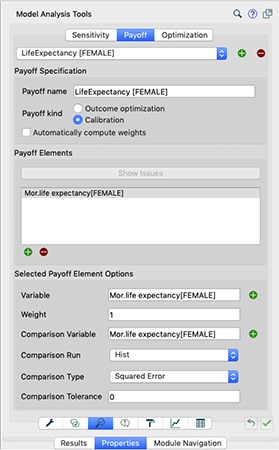
Disons que nous voulons optimiser l’espérance de vie moyenne. Dans l’écran principal des paramètres du modèle, cliquez sur le bouton de l’objectif en bas. Entrez les paramètres dans l’onglet Payoff comme dans l’image ci-dessous.

Ensuite, sur l’onglet « Optimization », entrez les paramètres comme dans l’image ci-dessous.

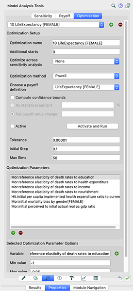
N.B. Nous fixons les simulations maximales à un niveau plus bas pour commencer, de sorte qu’en cas d’erreurs importantes, nous n’attendons pas trop longtemps. Ces simulations peuvent être réglées (fixées à un niveau plus haut) pour un calibrage plus fin, par la suite. Lorsque vous terminez, cliquez sur OK pour confirmer. Ensuite, ajoutez l’ensemble de paramètres souhaités. En cas d’élasticité de la mortalité illustrée ici, l’échelle appropriée serait [-0,5,-0,05]. Différents paramètres nécessitent des échelles différentes. Les ajustements, hors de portée, doivent être vérifiés et notés. Par exemple, l’ajustement des paramètres de temps nécessiterait généralement des valeurs positives plus importantes (par exemple 1,2… 20 ans). Lorsque vous êtes satisfait des paramètres, vérifiez les années de simulation et assurez-vous qu’elles se situent dans la fourchette des données historiques que vous essayez de faire correspondre. Puis, cliquez sur « Run »

N.B. Si vous ne disposez pas de données complètes sur la durée de la simulation, vous devrez raccourcir la durée de votre simulation. S’il y a des espaces entre les deux et que Stella les lit comme des zéros, vous devrez interpoler manuellement dans Excel.

Si l’ajustement est mauvais, il pourrait y avoir un problème avec l’entrée également. Attention aux extrémités, elles peuvent ne pas être la valeur idéale, et il peut être préférable de laisser une valeur plus raisonnable que d’avoir un calibrage parfait. De plus, avec le reste du calibrage dans le secteur et dans le modèle, les valeurs devraient de toute façon être ajustées plus tard.

Pour une meilleure compréhension, vous pouvez également analyser les limites de confiance (confidence bounds) : un outil utile pour comprendre la solidité des résultats du calibrage.

Footnotes

[1] Forrester, J W. 1961. Industrial Dynamics. Cambridge MA: Productivity Press.

[2] Barlas, Y. 1996. “Formal Aspects of Model Validity and Validation in System Dynamics.” System Dynamics Review 12, (3): 183–210.

[3] Forrester, J W, and P M Senge. 1980. “Tests for building confidence in System Dynamics models.” TIMS Studies in the Management Sciences 14: 201–28.

Richardson, G P, and III Alexander L Pugh. 1981. Introduction to System Dynamics Modeling with Dynamo. Waltham: Pegasus Communications.

Sterman, J 2000. Business Dynamics. Irwin/McGraw-Hill.

[4] The summary statistics can be reported for any series for which we have data.

[5] Sterman, J. 1984. “Appropriate summary statistics for evaluating the historical fit of System Dynamics Models.” Dynamica 10 (2): 51–66.

[6] Sterman, J. 1984. “Appropriate summary statistics for evaluating the historical fit of System Dynamics Models.” Dynamica 10 (2): 51–66.

Oliva, R. 2003. “Model calibration as a testing strategy for System Dynamics Models.” European Journal of Operational Research 151: 553–68.

[7] Powell, M J D. 2009. The BOBYQA Algorithm for Bound Constrained Optimization Without Derivatives. Department of Applied Mathematics; Theoretical Physics, Cambridge University.

[8] Homer, J B. 2012. “Partial-model testing as a validation tool for System Dynamics (1983).” System Dynamics Review 28 (3): 281–94.

Oliva, R. 2003. “Model calibration as a testing strategy for System Dynamics Models.” European Journal of Operational Research 151: 553–68.